── Attaching core tidyverse packages ──────────────────────── tidyverse 2.0.0 ──
✔ dplyr     1.1.4     ✔ readr     2.1.5
✔ forcats   1.0.0     ✔ stringr   1.5.1
✔ ggplot2   3.5.1     ✔ tibble    3.2.1
✔ lubridate 1.9.3     ✔ tidyr     1.3.1
✔ purrr     1.0.2
── Conflicts ────────────────────────────────────────── tidyverse_conflicts() ──
✖ dplyr::filter() masks stats::filter()
✖ dplyr::lag()    masks stats::lag()
ℹ Use the conflicted package (<http://conflicted.r-lib.org/>) to force all conflicts to become errorsA Grammar of Graphics
Introduction to ggplot2
18 septembre 2024
Workflow

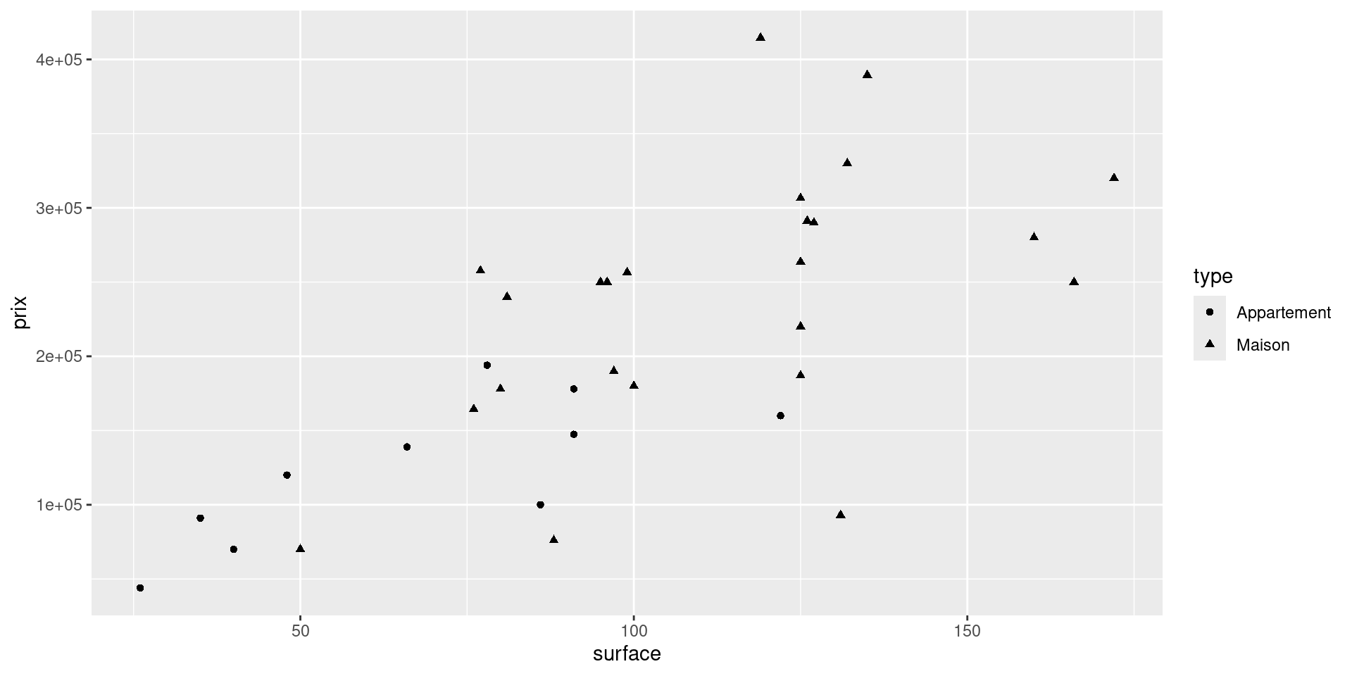
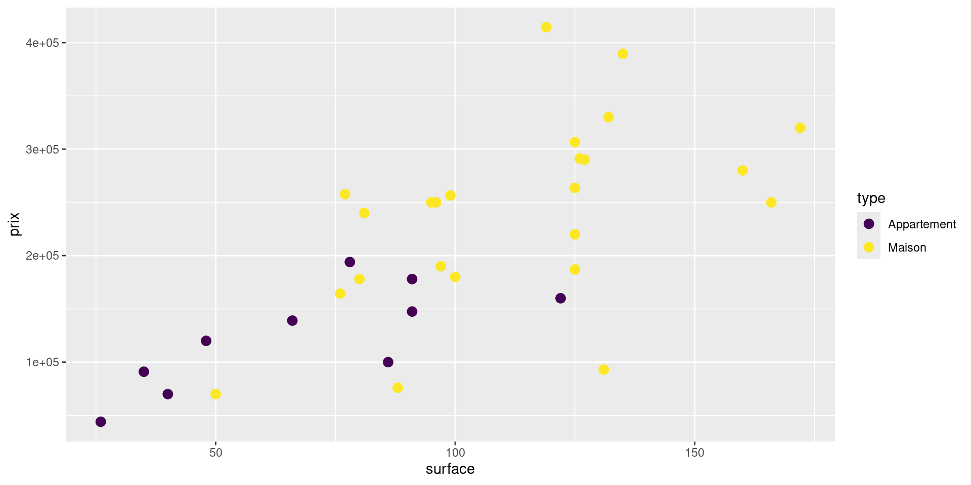
Scatterplot

Boxplot

Size aesthetic

Let’s break it down

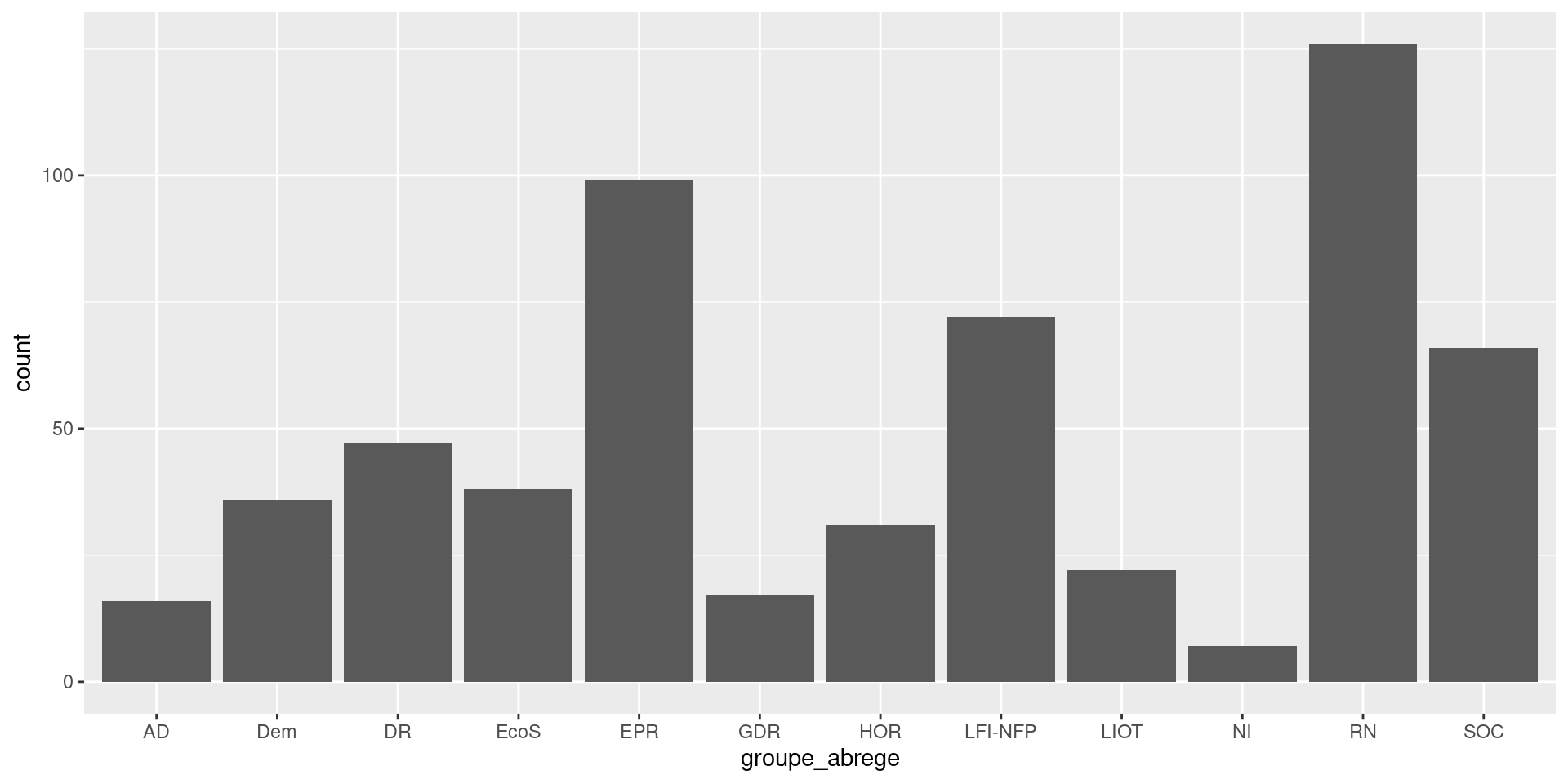
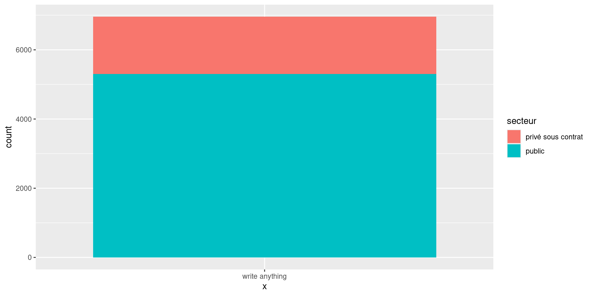
Barplot

Boxplot
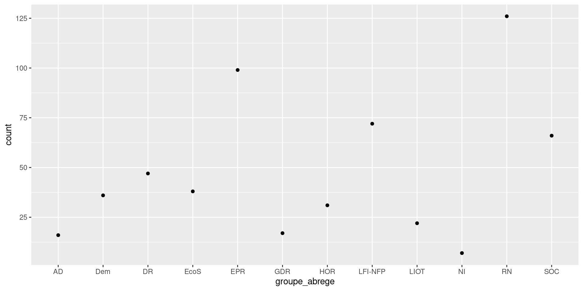
Scatterplot
Density 2D

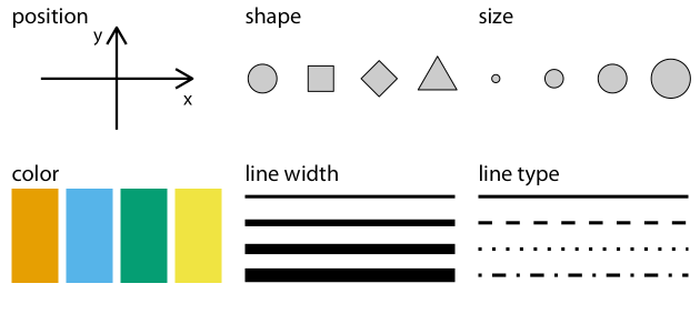
Aesthetics
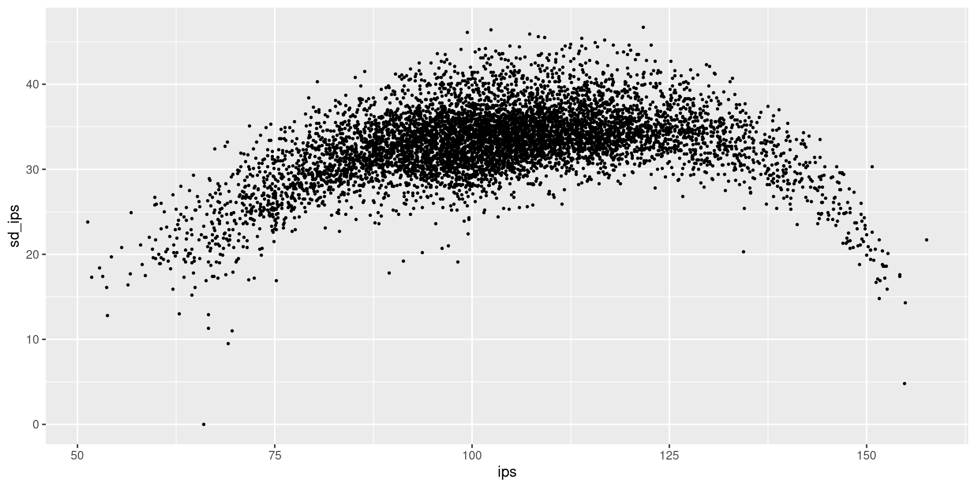
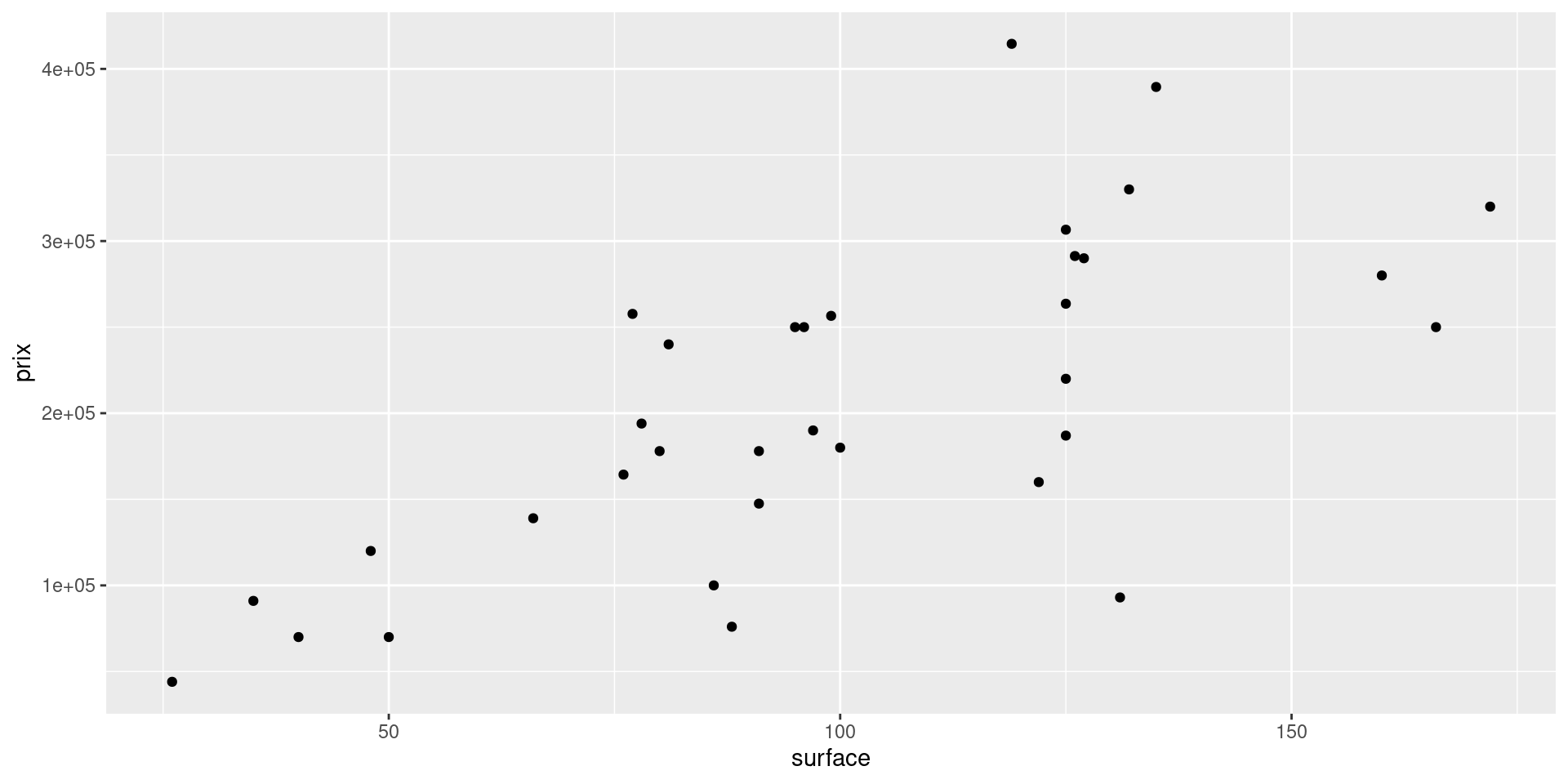
Raw scatterplot

Setting alpha

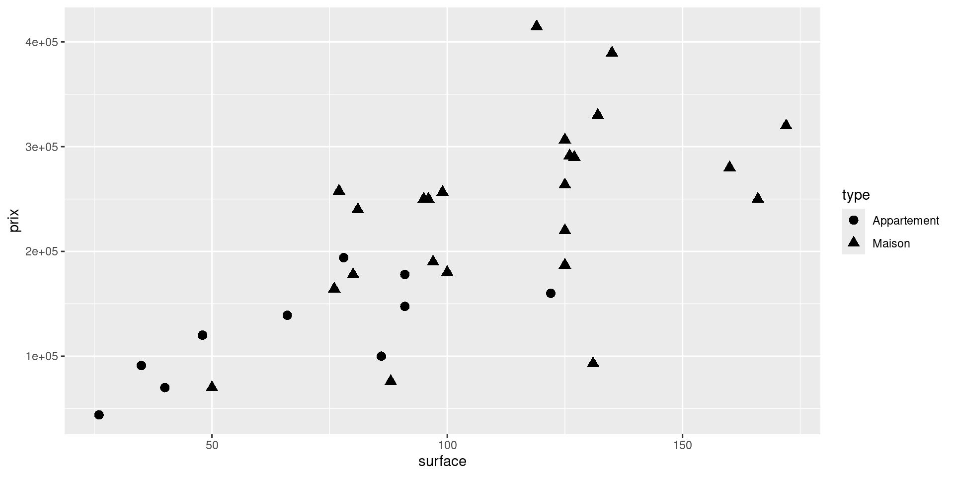
Setting size
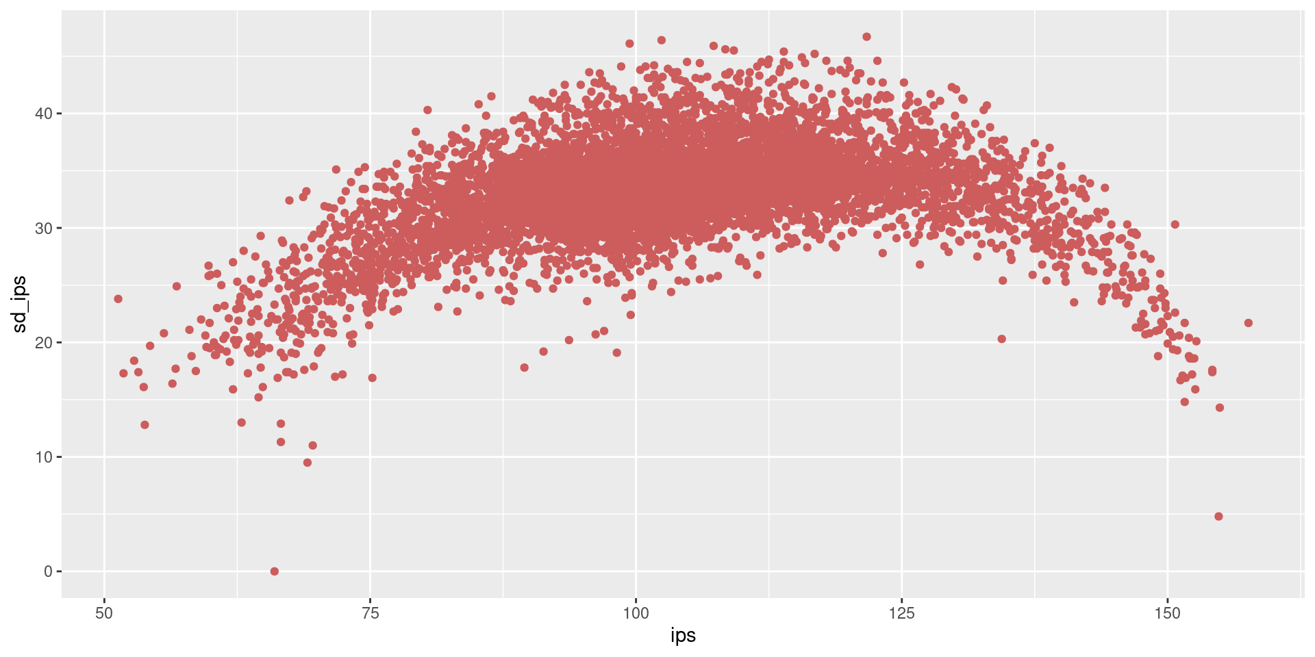
Setting color
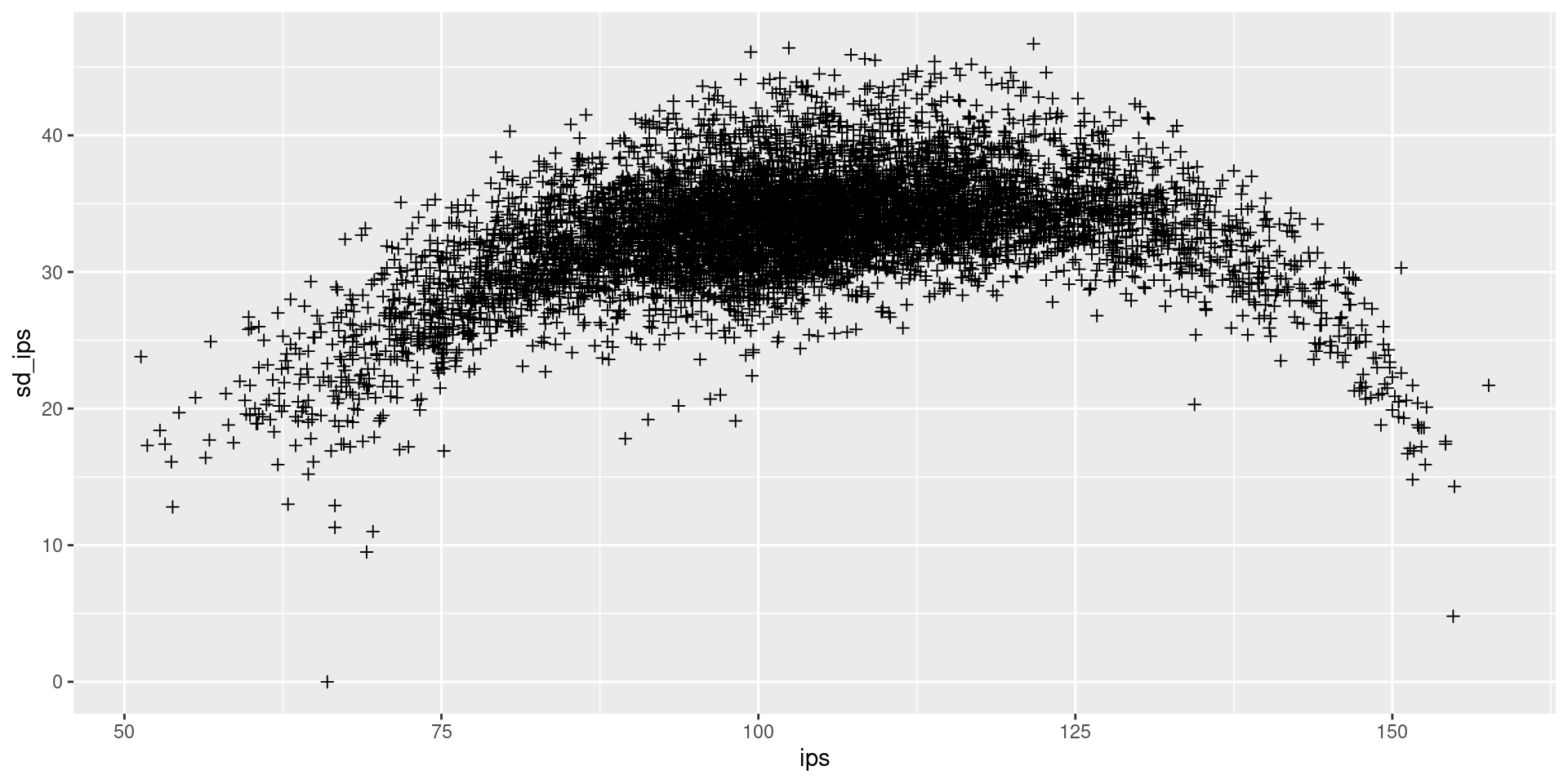
Setting shape
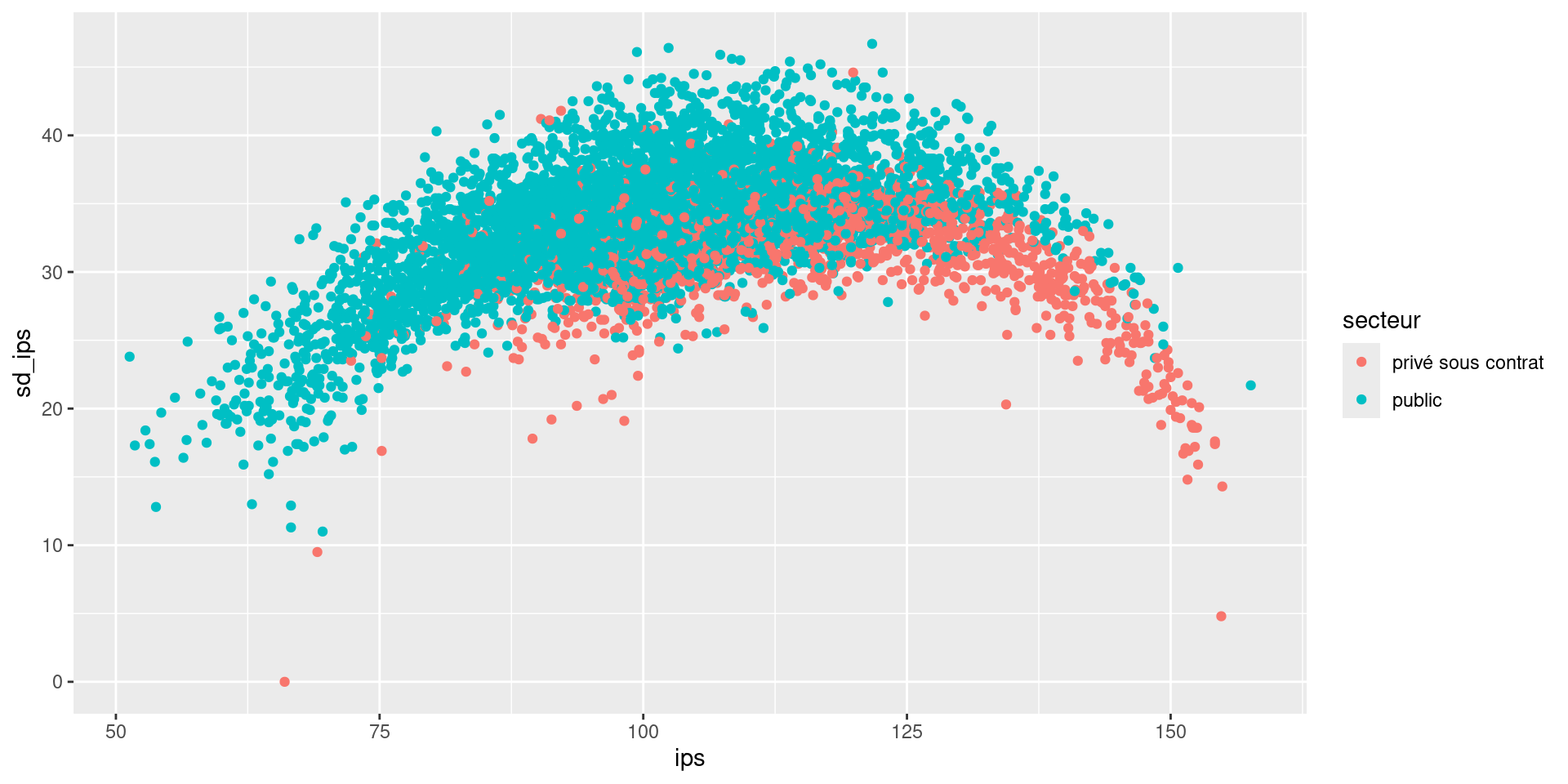
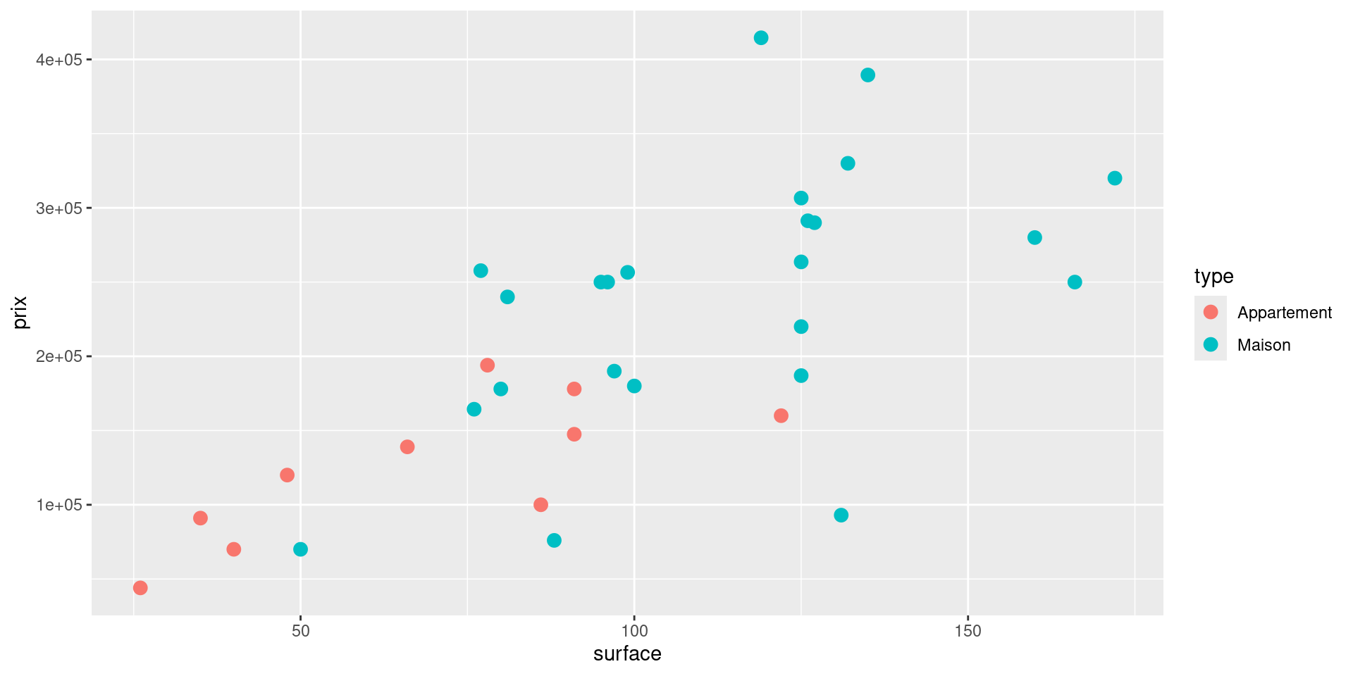
Mapping color
Maping shape
Mapping and setting
geom_X()

stat_X()

layer()
Exploring combinations
point
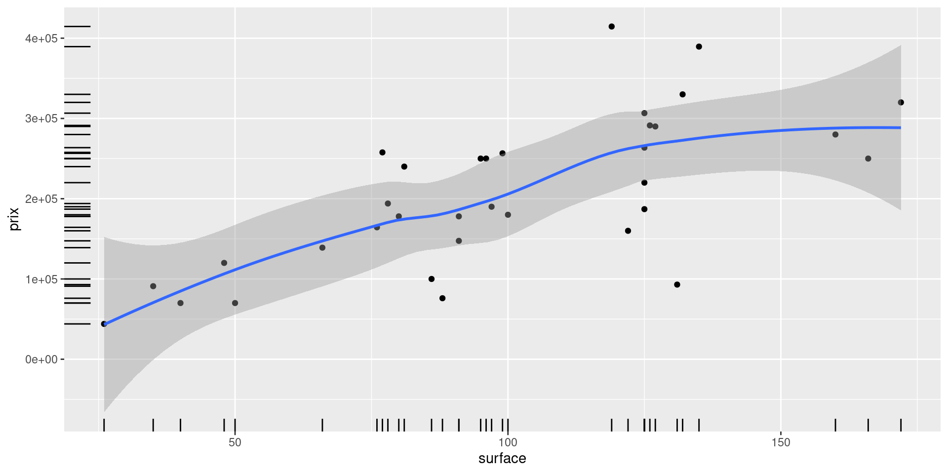
point + smooth

point + smooth + rug
Color aesthetic
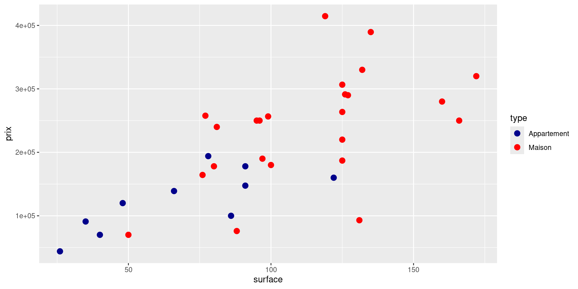
Scale color manual
Scale color viridis
Cartesian coordinates
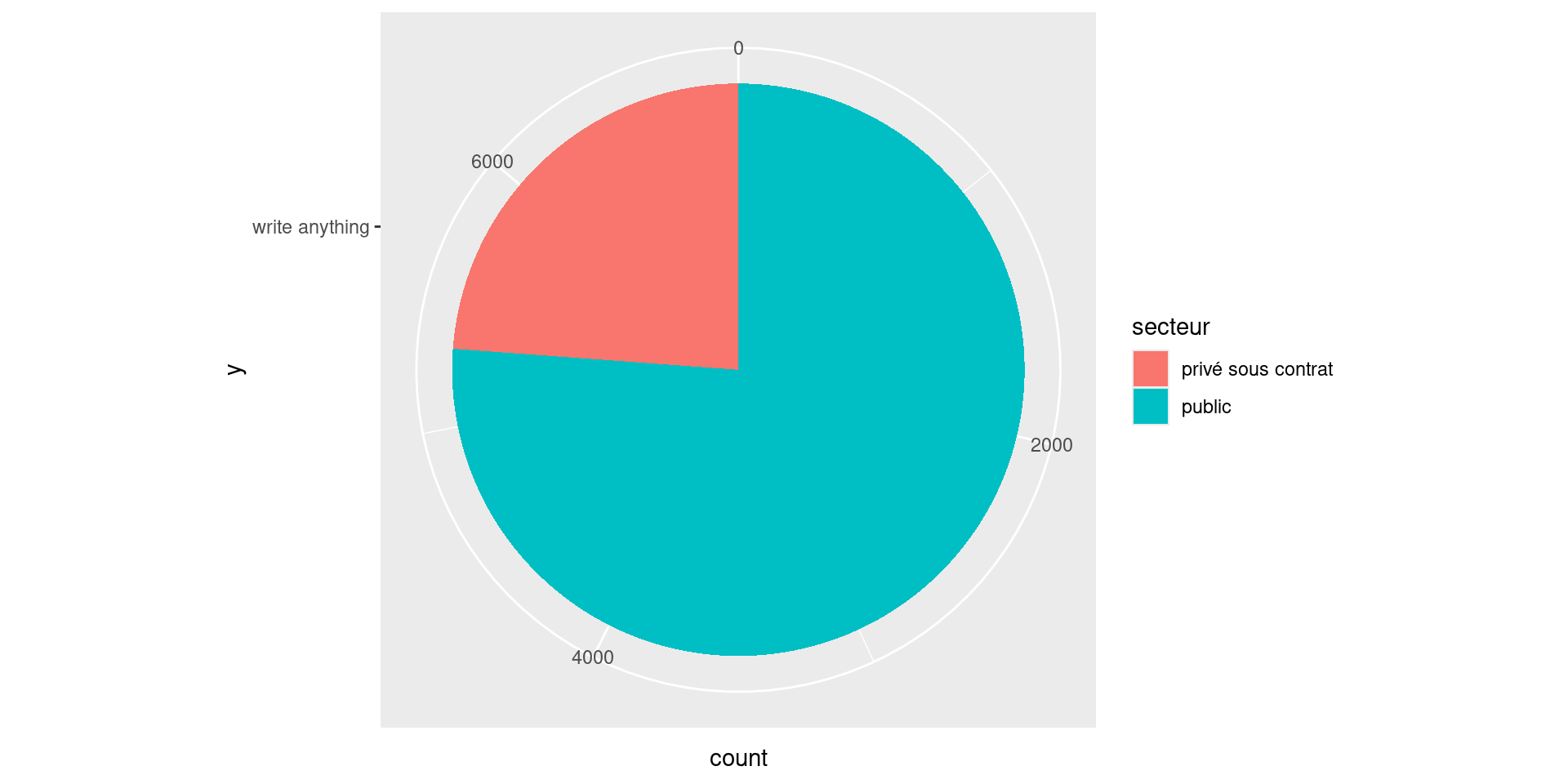
Polar coordinates
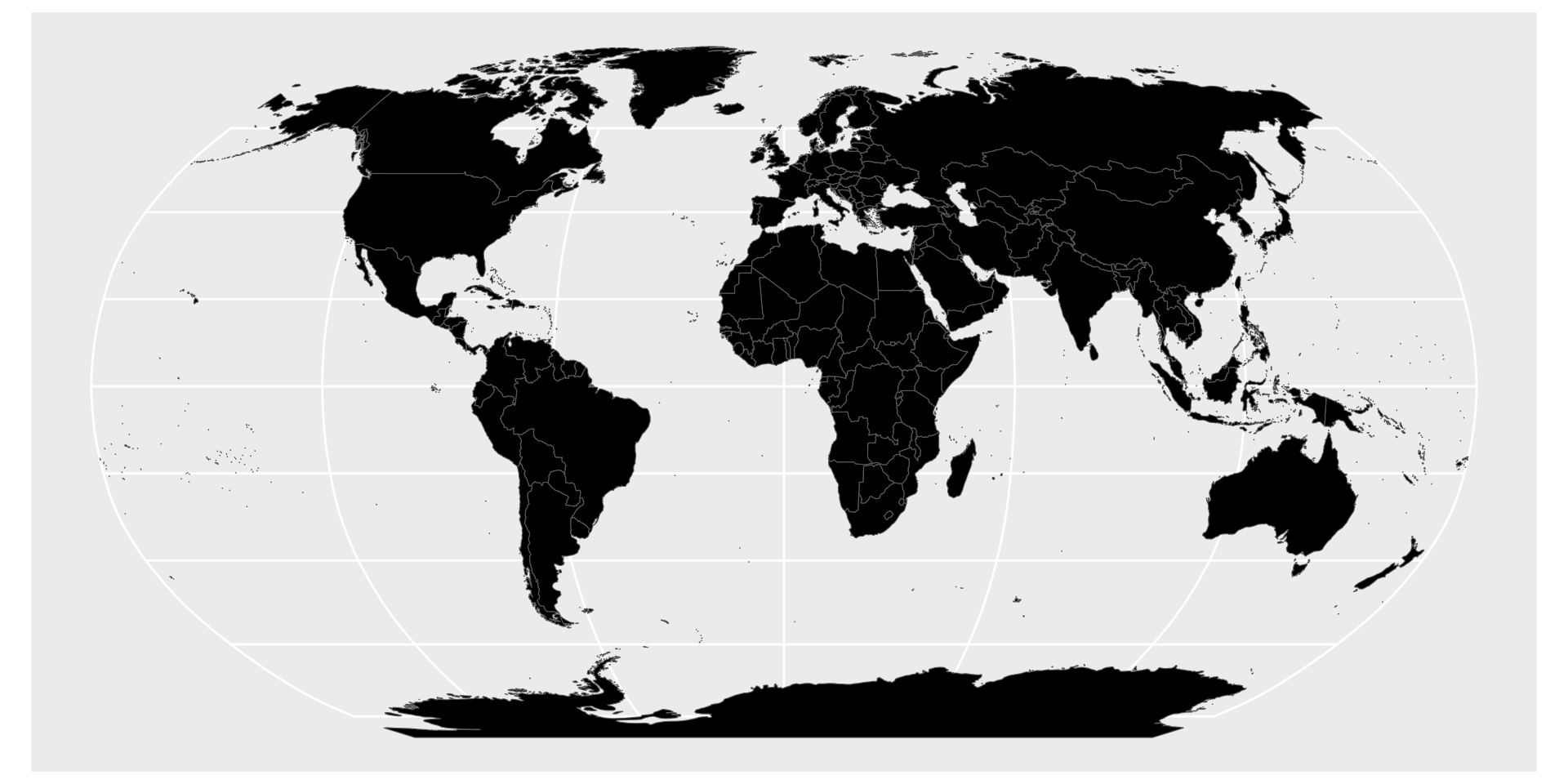
Cartographic coordinates
Another one
First example

Meaningful example
Code
d = fs::path_home("these", "data", "eec") |>
  arrow::open_dataset() |>
  filter(rgi == 1,
         !is.na(acteu)) |>
  select(sexe, ag, acteu, csp, csa, santgen) |>
  mutate(cs = coalesce(csp, csa),
         cs = if_else(cs %in% c("10", "11", "12", "13"), "10", cs)) |>
  collect()

d |>
  filter(between(ag, 20, 80)) |>
  group_by(ag, cs, santgen) |>
  summarise(n = n()) |>
  mutate(pct = n / sum(n)) |>
  ungroup() |>
  pivot_wider(names_from = santgen, values_from = c(pct, n), values_fill = 0) |>
  mutate(good = pct_1 + pct_2) |>
  select(ag, cs, good) |>
  ggplot() +
  geom_smooth(aes(x = ag, y = good)) +
  facet_wrap(~cs) +
  labs(x = "",
       y = "Proportion de personnes en bonne santé") +
theme_bw() 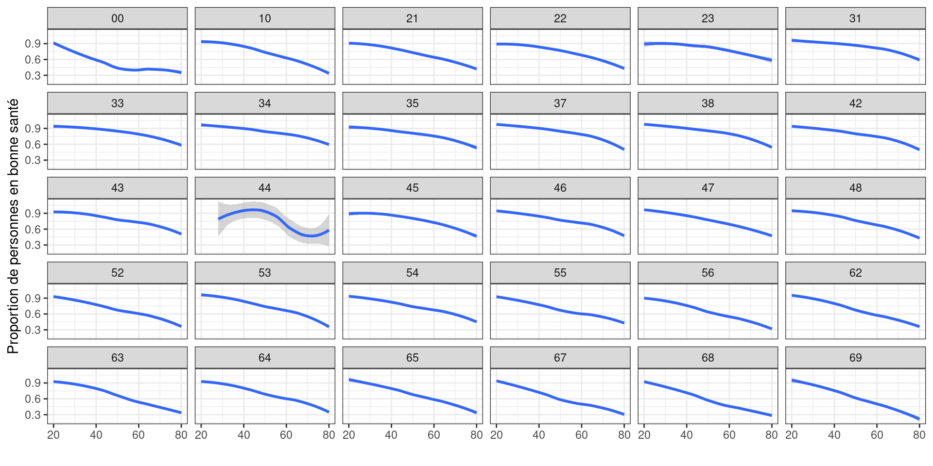
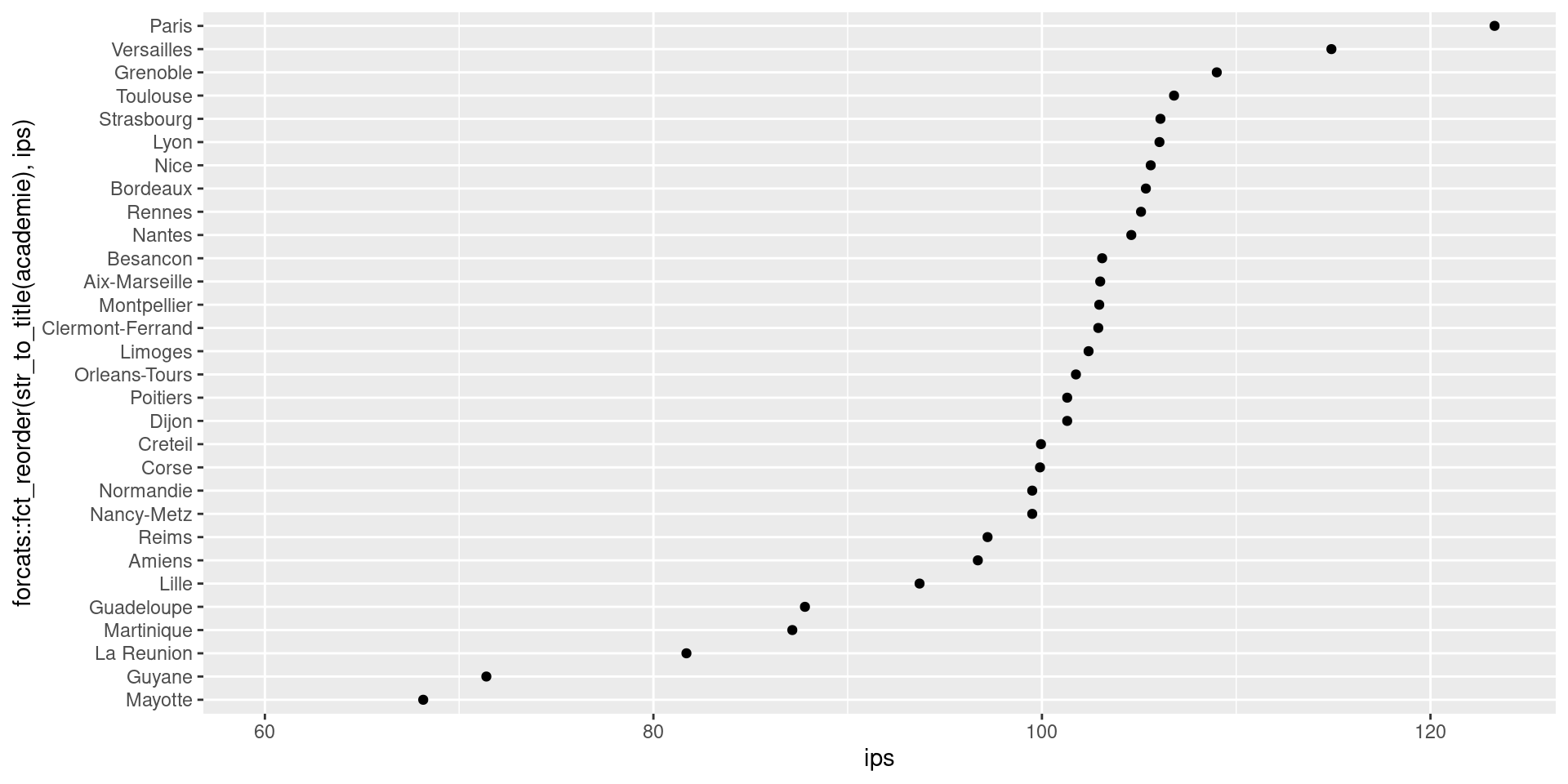
A plot to dress up
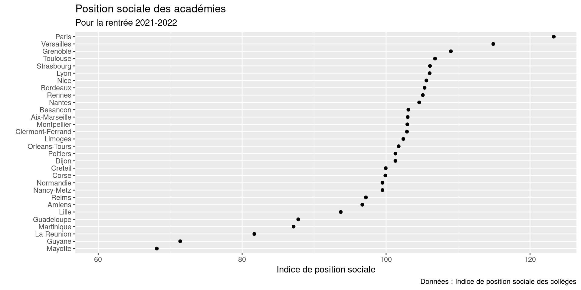
labs()
Code
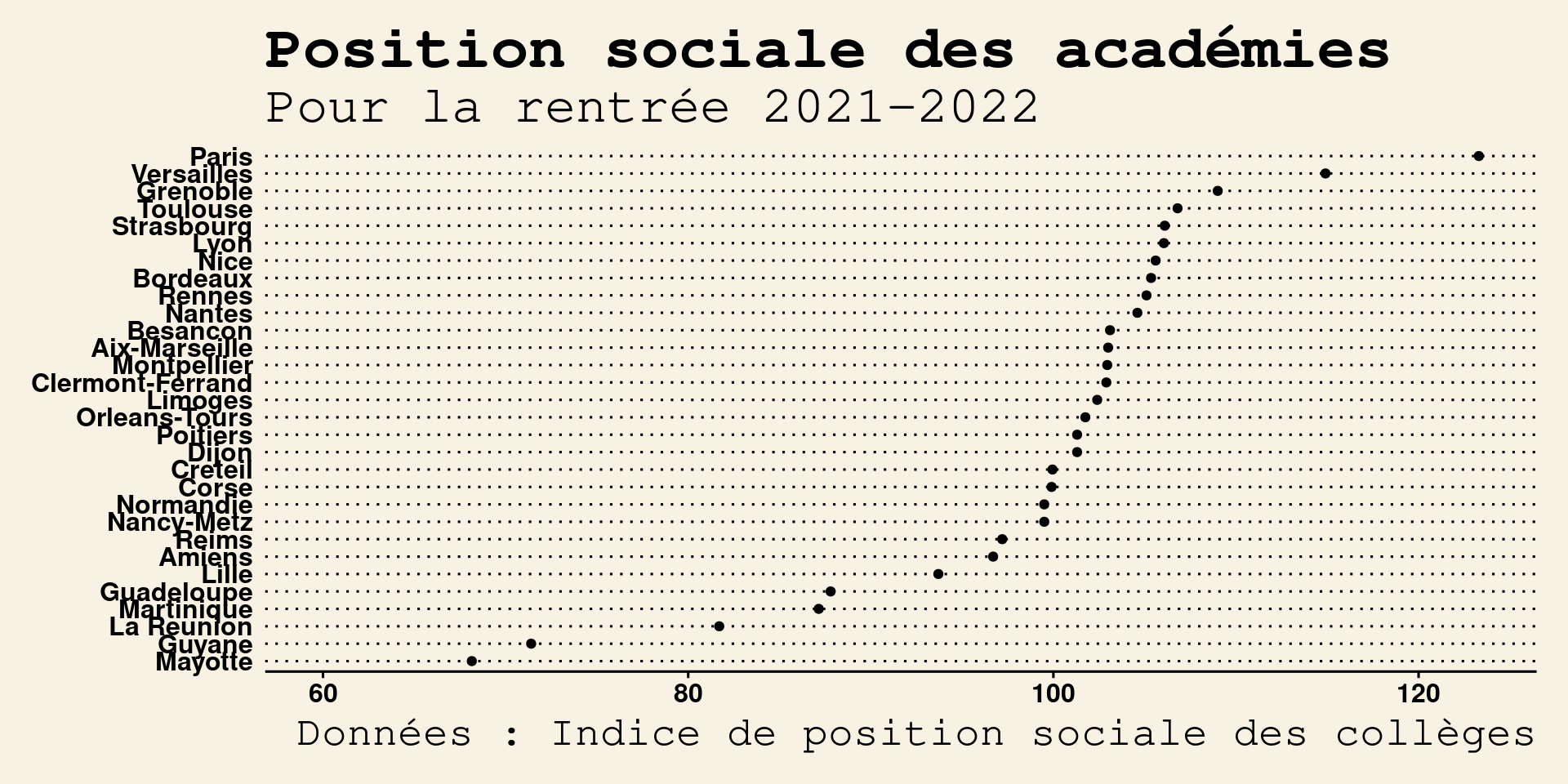
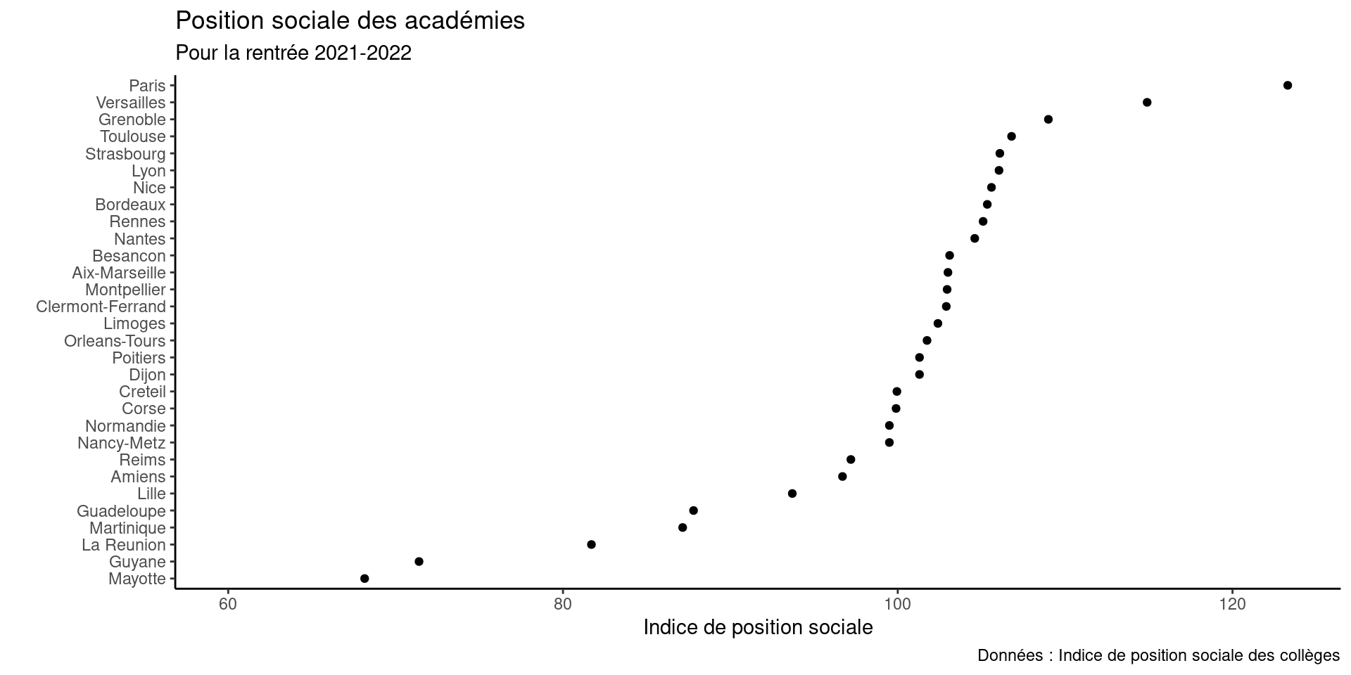
ggplot(ips, aes(y = forcats::fct_reorder(str_to_title(academie), ips),
                    x = ips)) +
  stat_summary(fun = "median", geom = "point") +
coord_cartesian(xlim = c(60, NA)) +
labs(x = "Indice de position sociale",
y = "",
title = "Position sociale des académies",
subtitle = "Pour la rentrée 2021-2022",
caption = "Données : Indice de position sociale des collèges")
Grey (default)
Classic
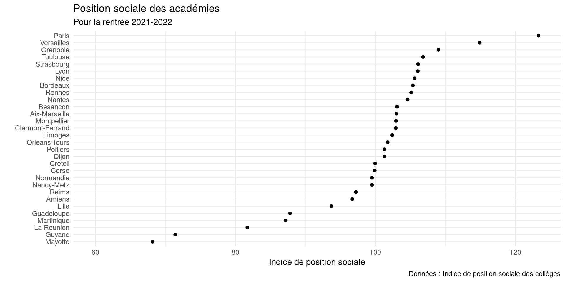
Minimal
WSJ