18 décembre 2024
https://ben18785.shinyapps.io/distribution-zoo/
rbinom(n = 10, size = 30, prob = 0.5)
[1] 15 13 15 11 16 21 19 14 15 12
rbinom(n = 10, size = 1, prob = 0.7)
[1] 1 1 1 1 1 1 1 0 1 1
rnorm(n = 10, mean = 2600, sd = 1000)
 [1] 2352.854 3789.456 2844.240 2103.881 3758.489 3057.468 4906.261 3556.442
 [9] 3885.535 3807.580
rpois(n = 10, lambda = 3)
[1] 0 8 4 3 5 3 6 2 5 4
rbeta(n = 10, shape1 = 7, shape2 = 3)
 [1] 0.5551196 0.4152760 0.5146809 0.8318127 0.6721343 0.8759235 0.7662018
 [8] 0.4818727 0.7812606 0.5406850
population = data.frame(revenu = rnorm(n = 100000, mean = 1300, sd = 600),
                        celibataire = rbinom(n = 100000, size = 1, prob = 0.35))
tibble::as_tibble(population)
# A tibble: 100,000 × 2
   revenu celibataire
    <dbl>       <int>
 1   865.           0
 2   102.           0
 3  2077.           1
 4   252.           0
 5   411.           0
 6  1248.           0
 7  1789.           0
 8   669.           1
 9  1078.           0
10  1180.           0
# ℹ 99,990 more rows
echantillon = dplyr::slice_sample(population, n = 31)
mean_revenu = mean(echantillon$revenu)
proportion_celibataires = sum(echantillon$celibataire == 1) / 31
echantillon |> as_tibble()
mean_revenu
proportion_celibataires
# A tibble: 31 × 2
   revenu celibataire
    <dbl>       <int>
 1  1454.           0
 2  1647.           1
 3   747.           0
 4  2049.           1
 5  1362.           1
 6  1786.           0
 7  1124.           0
 8   652.           0
 9  2182.           0
10  1380.           0
# ℹ 21 more rows
[1] 1384.903
[1] 0.2258065
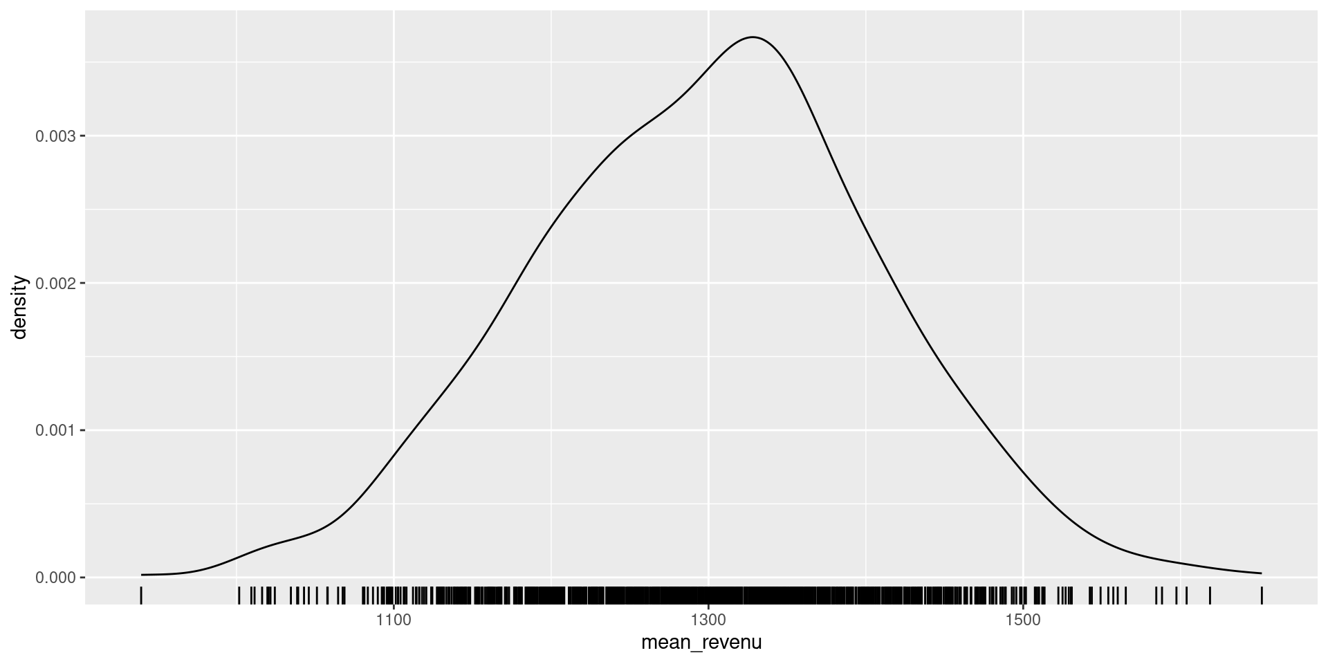
echantillons = replicate(n = 1000, dplyr::slice_sample(population, n = 31), simplify = FALSE)
params_echantillons = purrr::map(echantillons, ~summarise(.x,
                                    mean_revenu = mean(revenu),
                                    proportion_celibataires = sum(celibataire == 1) / 31)) |>
  list_rbind()
ggplot(params_echantillons) +
  geom_density(aes(x = mean_revenu)) +
  geom_rug(aes(x = mean_revenu))
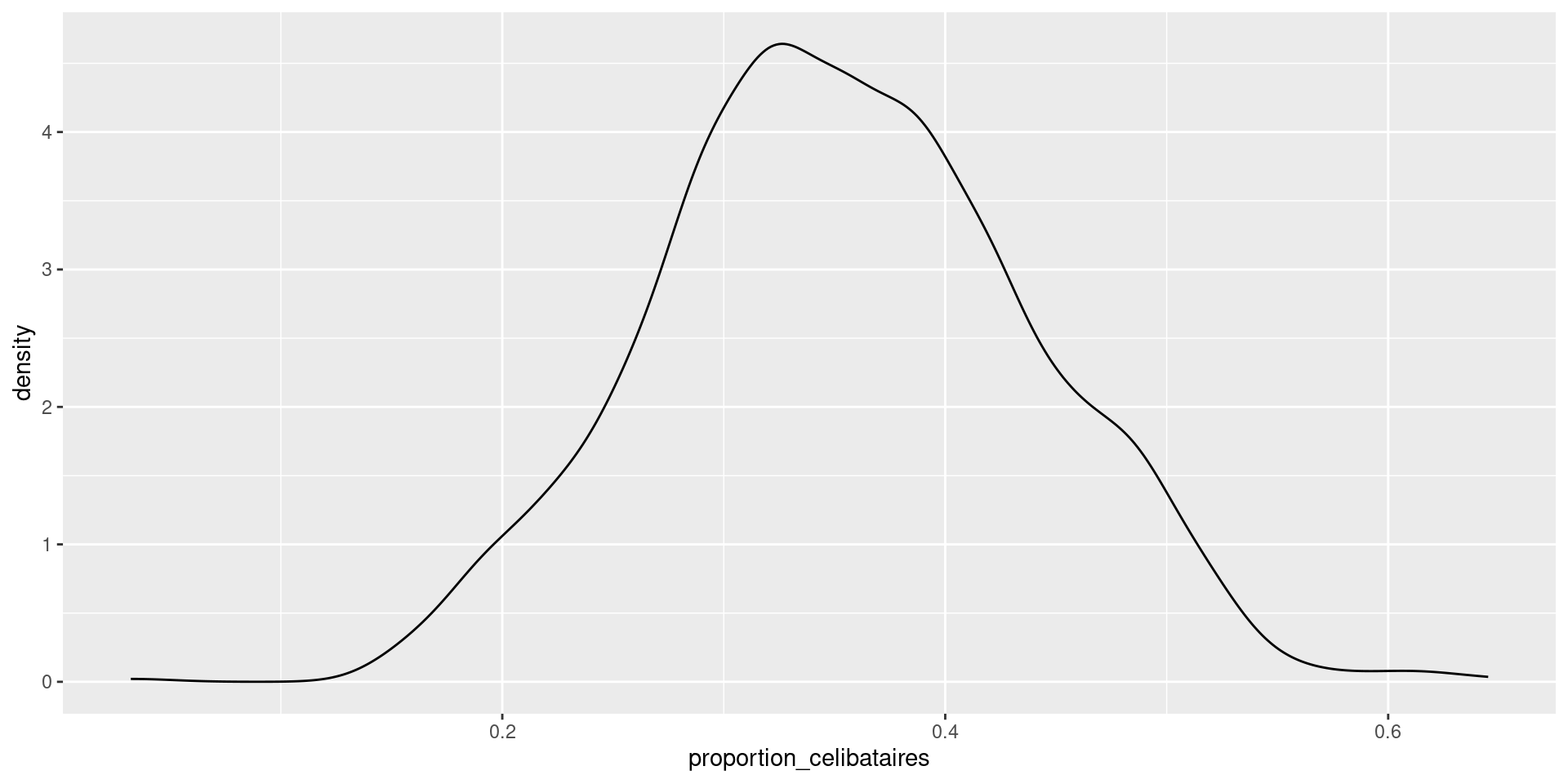
ggplot(params_echantillons) +
  geom_density(aes(x = proportion_celibataires))